高斯玻色采样(Gaussian Boson Sampling)

数学背景

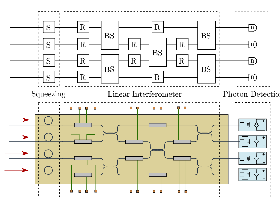
高斯玻色采样(GBS)可以作为玻色采样的一种变体，不同之处在于输入的量子态是高斯压缩态而不是离散的Fock态。 压缩态是高斯态的一种，高斯态指的是这个量子态对应的Wigner函数是高斯分布，比如相干态。 单模压缩态的Wigner函数对应的高斯分布在 \(X\)，\(P\) 两个正交分量上会压缩或者拉伸，单模压缩态可以将压缩门作用到真空态上得到，也可以用下面的Fock态基矢展开[2]，需要注意的是这里的Fock态光子数从0到无穷大取偶数，因此输出的量子态的空间是无限大且只包含偶数光子数的Fock态空间。

\[ \ket{\mathrm{sq}_R} = \frac{1}{\sqrt{\cosh r}} \sum_{m=0}^{\infty} (-\tanh r)^m \frac{\sqrt{(2m)!}}{2^m m!} \ket{2m} \]

GBS采样概率的理论计算和玻色采样类似，不同之处在于对粒子数分辨探测器和阈值探测器两种情况，分别需要用hafnian函数和torotonian函数来计算。

1. 粒子数分辨探测器

在探测端口使用粒子数分辨探测器时对应数学上需要计算hafnian函数， 对于 \(2m\times 2m\) 对称矩阵 \(A\) 的hafnian定义如下[3]，

\[ \mathrm{haf}(\boldsymbol{A}) = \sum_{M \in \mathrm{PMP}(n)} \prod_{(i,j) \in M} A_{i,j} \]

这里PMP表示所有完美匹配排列的集合，当 \(n=4\) 时，\(PMP(4) = {(0,1)(2,3),(0,2)(1,3),(0,3)(1,2)}\)，对应的矩阵 \(B\) 对应的hafnian如下

\[ \mathrm{haf}(B) = B_{0,1}B_{2,3}+B_{0,2}B_{1,3} + B_{0,3}B_{1,2} \]

在图论中，hafnian计算了图 \(G\) 对应的邻接矩阵A描述的图的完美匹配数(这里图 \(G\) 是无权重，无环的无向图)，比如邻接矩阵 \(A =\begin{pmatrix} 0&1&1&1\\ 1&0&1&1\\ 1&1&0&1\\ 1&1&1&0 \end{pmatrix}\)，haf(A)=3，对应的完美匹配图如下。

当计算的图是二分图时，得到的hafnian计算结果就是permanent。

\[\begin{split} \mathrm{haf} \left( \begin{bmatrix} 0 & \boldsymbol{W} \\ \boldsymbol{W}^T & 0 \end{bmatrix} \right) = \mathrm{per}(\boldsymbol{W}) \end{split}\]

因此任何计算hafnian的算法也可以用来计算permanent，同样的计算hafnian也是 \(\#P\) 难问题。

对于粒子数探测器，输出的Fock态 \(S = (s_1, s_2,..,s_m)\) 时，对应的 \(s_i=0,1,2...\)， 输出态的概率理论计算如下

\[ \Pr(S) = \frac{1}{\sqrt{\det(\boldsymbol{Q})}} \frac{\mathrm{Haf}(\boldsymbol{\mathcal{A}}_S)}{s_1! s_2! \cdots s_m!} \]

这里 \(Q,A,X\) 的定义如下，

\[\begin{split} \begin{aligned} \boldsymbol{Q} &:= \boldsymbol{\Sigma} + \mathbb{1}/2, \\ \boldsymbol{\mathcal{A}} &:= \boldsymbol{X} (\mathbb{1} - \boldsymbol{Q}^{-1}) \\ \boldsymbol{X} &:= \begin{bmatrix} 0 & \mathbb{1} \\ \mathbb{1} & 0 \end{bmatrix}. \end{aligned} \end{split}\]

\(Q,A\) 由输出量子态的协方差矩阵 \(\Sigma\) 决定 ( \(\Sigma\) 描述的是 \(a,a^+\) 的协方差矩阵)，子矩阵 \(A_s\) 由输出的Fock态决定，具体来说取矩阵 \(A\) 的 \(i, i+m\) 行和列并且重复 \(s_i\) 次来构造 \(A_s\) 。 如果 \(s_i=0\)，那么就不取对应的行和列，如果所有的 \(s_i=1\), 那么对应的子矩阵 \(A_s = A\)。

考虑高斯态是纯态的时候， 矩阵\(A\)可以写成直和的形式，\(A = B \oplus B^*\), \(B\) 是 \(m\times m\) 的对称矩阵。这种情况下输出Fock态的概率如下

\[ \Pr(S) = \frac{1}{\sqrt{\det(\boldsymbol{Q})}} \frac{|\mathrm{Haf}(\boldsymbol{{B}}_S)|^2}{s_1! s_2! \cdots s_m!} \]

这里的子矩阵 \(B_s\) 通过取 \(i\) 行和 \(i\) 列并且重复 \(s_i\) 次来构造，同时这里hafnian函数计算的矩阵维度减半，可以实现概率计算的加速。

当所有模式输出的光子数 \(s_i = 0,1\) 时，对应的 \(A_s\) 是A的子矩阵，也对应到邻接矩阵A对应的图 \(G\) 的子图，利用这个性质可以解决很多子图相关的问题，比如稠密子图，最大团问题等。

2. 阈值探测器

使用阈值探测器时对应的输出Fock态概率 \(S = (s_1, s_2,..,s_m)，s_i\in \{0,1\}\)，此时理论概率的计算需要用到Torontonian函数[4]

\[ p(\boldsymbol{S}) = \frac{\mathrm{Tor}[\boldsymbol{O}_{(S)}]}{\sqrt{\det(\boldsymbol{\Sigma})}} \]

\[ \mathrm{Tor}[\boldsymbol{O}_{(S)}] = \mathrm{Haf}[\boldsymbol{X}\boldsymbol{O}_{(S)}] + \sum_{S' \in \mathcal{C}_S} \frac{\mathrm{Haf}[\boldsymbol{X}\boldsymbol{O}_{(S')}]}{s'_1! \dots s'_\ell!} \]

这里 \(O_s = I-(\Sigma^{-1})_s\)，直观上来看对于阈值探测器对应的特定的Fock态输出只需要将粒子数分辨探测器对应的多个Fock态概率求和即可。

代码演示

下面简单演示6个模式的高斯玻色采样任务

import deepquantum as dq
import numpy as np

squeezing = [1] * 6
unitary = np.eye(6)
gbs = dq.photonic.GaussianBosonSampling(nmode=6, squeezing=squeezing, unitary=unitary)
gbs()
gbs.draw()  # 画出采样线路

设置粒子数分辨探测器开始采样并输出Fock态结果

gbs.detector = 'pnrd'
result = gbs.measure(shots=1024, mcmc=True)
print(result)

Using MCMC method to sample the final states!

chain 1: 100%|███████████████████████████████| 203/203 [00:00<00:00, 236.69it/s]
chain 2: 100%|███████████████████████████████| 203/203 [00:00<00:00, 548.63it/s]
chain 3: 100%|███████████████████████████████| 203/203 [00:00<00:00, 652.31it/s]
chain 4: 100%|██████████████████████████████| 203/203 [00:00<00:00, 1000.01it/s]
chain 5: 100%|██████████████████████████████| 207/207 [00:00<00:00, 1293.74it/s]

{|000000>: 779, |020200>: 48, |002002>: 121, |002200>: 10, |000002>: 28, |002000>: 11, |000202>: 27}

设置阈值探测器开始采样并输出Fock态结果

gbs.detector = 'threshold'
result = gbs.measure(shots=1024, mcmc=True)
print(result)

Using MCMC method to sample the final states!

chain 1:   0%|                                          | 0/203 [00:00<?, ?it/s]

chain 1: 100%|███████████████████████████████| 203/203 [00:00<00:00, 858.50it/s]
chain 2: 100%|█████████████████████████████| 203/203 [00:00<00:00, 18455.08it/s]
chain 3: 100%|█████████████████████████████| 203/203 [00:00<00:00, 67671.57it/s]
chain 4: 100%|█████████████████████████████| 203/203 [00:00<00:00, 67676.95it/s]
chain 5: 100%|█████████████████████████████| 207/207 [00:00<00:00, 41395.10it/s]

{|100100>: 23, |100000>: 50, |100101>: 14, |011001>: 15, |000100>: 76, |110001>: 6, |111001>: 5, |010001>: 16, |010101>: 9, |011100>: 9, |101010>: 18, |011111>: 3, |010100>: 27, |011110>: 5, |000011>: 31, |110000>: 26, |100010>: 30, |001011>: 12, |110110>: 6, |000111>: 15, |101110>: 10, |011101>: 13, |111101>: 4, |001100>: 27, |101000>: 38, |000110>: 26, |110100>: 9, |100001>: 17, |100110>: 8, |010110>: 12, |100111>: 7, |101100>: 14, |110101>: 5, |010000>: 54, |100011>: 13, |000000>: 53, |001110>: 13, |001010>: 30, |011011>: 4, |000010>: 41, |011000>: 14, |000101>: 15, |111100>: 6, |111000>: 17, |010010>: 23, |001001>: 23, |111110>: 4, |111111>: 1, |101101>: 6, |010111>: 5, |000001>: 31, |010011>: 10, |101111>: 3, |001000>: 22, |110011>: 6, |001111>: 5, |001101>: 5, |111011>: 2, |110010>: 7, |101001>: 12, |011010>: 5, |101011>: 2, |111010>: 4, |110111>: 2}

附录

[1] Lvovsky, Alexander I. “Squeezed light.” Photonics: Scientific Foundations, Technology and Applications 1 (2015): 121-163.

[2]Bromley, Thomas R., et al. “Applications of near-term photonic quantum computers: software and algorithms.” Quantum Science and Technology 5.3 (2020): 034010.

[3]Quesada, Nicolás, Juan Miguel Arrazola, and Nathan Killoran. “Gaussian boson sampling using threshold detectors.” Physical Review A 98.6 (2018): 062322.

[4]J. M. Arrazola and T. R. Bromley, Physical Review Letters 121, 030503 (2018)