复杂纠缠态制备

前面介绍了单模线路结合时域复用方法制备简单的纠缠态，包括EPR态和GHZ态，这里介绍多模线路结合时域复用方法制备复杂的纠缠态。

案例一：扩展EPR的制备

第一种纠缠态的制备线路如下图所示， 由东京大学组提出[1]， 通过两模线路结合延时线圈，实现了四个测量结果的纠缠，即实现了相邻两个时刻的两组测量结果纠缠。

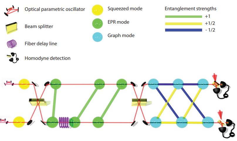
首先两组连续变量压缩光经过一个 \(1:1\) 的分束器形成纠缠，第二模的量子态经过延时线圈和第二个时刻的第一模中的量子态再通过分束器纠缠，从而使得 输出的相邻两个时刻的两组测量结果纠缠起来。

下面给出这种纠缠态制备线路的理论分析以及使用DeepQuantum代码复现。

理论分析

这里我们在薛定谔表象中研究量子态如何经过一系列光量子门后演化到纠缠态。

1.初态

\(k\) 时刻的初态可以表示为

\[ \psi_k = |x=0\rangle^A_k|p=0\rangle^B_k = \int_{-\infty}^{+\infty}|x=0\rangle^A_k|x=a_k\rangle^B_k da_k \]

那么考虑多个时刻的量子态初态为

\[ \Psi_0 = \prod_k \int_{-\infty}^{+\infty}|x=0\rangle^A_k|x=a_k\rangle^B_k da_k \]

\(k\) 表示不同时刻的指标。

2.第一个分束器

经过第一个\(1:1\) 分束器，相同时刻实现空间上的纠缠

\[ \Psi_1 = \hat{BS} \Psi_0 = \prod_k \int_{-\infty}^{+\infty}|x=\frac{a_k}{\sqrt{2}}\rangle^A_k |x=\frac{a_k}{\sqrt{2}}\rangle^B_k da_k \]

具体可以写成

\[ \Psi_1 =\int_{-\infty}^{+\infty}\int_{-\infty}^{+\infty}\int_{...}|x=\frac{a_1}{\sqrt{2}}\rangle^A_1 |x=\frac{a_1}{\sqrt{2}}\rangle^B_1 |x=\frac{a_2}{\sqrt{2}}\rangle^A_2 |x=\frac{a_2}{\sqrt{2}}\rangle^B_2 da_1da_2...... \]

3. 延时线圈

作用在模式B上的延时线圈仅仅起到延时作用，没有分束器起作用。

\[ \Psi_2 =\int_{-\infty}^{+\infty}\int_{-\infty}^{+\infty}\int_{...}|x=\frac{a_1}{\sqrt{2}}\rangle^A_1 |x=\frac{a_1}{\sqrt{2}}\rangle^B_2 |x=\frac{a_2}{\sqrt{2}}\rangle^A_2 |x=\frac{a_2}{\sqrt{2}}\rangle^B_3 da_1da_2...... \]

4. 第二个分束器

经过第二个\(1:1\) 分束器，相同时刻实现空间上的纠缠。

\[ \Psi_2 =\int_{-\infty}^{+\infty}\int_{-\infty}^{+\infty}\int_{...}|x=\frac{a_1}{\sqrt{2}}\rangle^B_1|x=\frac{a_1}{\sqrt{2}}\rangle^A_1 |x=\frac{1}{2}(a_2-a_1)\rangle^B_2 |x=\frac{1}{2}(a_2+a_1)\rangle^A_2 |x=\frac{1}{2}(a_3-a_2)\rangle^B_3 |x=\frac{1}{2}(a_3+a_2)\rangle^A_3 da_1da_2da_3...... \]

考虑相邻两次的测量结果，

\[ \frac{1}{2}(a_k-a_{k-1}) + \frac{1}{2}(a_k+a_{k-1}) + \frac{1}{2}(a_{k+1}-a_{k}) - \frac{1}{2}(a_{k+1}+a_{k}) = 0 \]

可以看到相邻的两次测量结果关联起来了，形成了四个量子态组成的纠缠态。

代码演示

import deepquantum as dq
import numpy as np
import torch

r = 6
nmode = 2
cir = dq.QumodeCircuitTDM(nmode=nmode, init_state='vac', cutoff=3)
cir.s(0, r=r)
cir.s(1, r=r)
cir.r(0, np.pi / 2)
cir.bs([0, 1], [np.pi / 4, 0])
cir.delay(1, ntau=1, inputs=[np.pi / 2, 0])
cir.bs([0, 1], [np.pi / 4, 0])
cir.homodyne_x(0)
cir.homodyne_x(1)
cir.to(torch.double)
cir()
cir.draw()

完成线路前向运行之后可以查看等效的线路

cir.draw(unroll=True)

shots = 20
cir(nstep=20)
samples = cir.samples
print(samples.mT)

tensor([[  -9.4332,   -6.7339],
        [ 347.3914,  363.5567],
        [ 644.8513,  -66.0994],
        [ 442.2943, -136.4661],
        [  31.7089, -274.1145],
        [ 122.4824,  364.8849],
        [  33.2360, -454.1305],
        [-145.6183,  275.2744],
        [ 145.0562,   15.4012],
        [  63.9466,  -96.5084],
        [ -26.7371,    5.8232],
        [ 131.8538,  152.7683],
        [ 223.9500,  -60.6742],
        [-104.0268, -267.3069],
        [-166.9784,  204.3499],
        [  21.8937,  -15.4776],
        [-389.8816, -396.2973],
        [-461.7313,  324.4476],
        [-105.4010,   31.8808],
        [-209.5396, -136.0182]], dtype=torch.float64)

计算相邻两次测量结果共四个结果的误差, 可以看到误差很小，因此可以认为它们相互纠缠起来。

size = int(shots / 2)
samples_reshape = samples.mT.reshape(size, 2, 2)
x_delta = []
for i in range(size):
    temp = samples_reshape[i].sum() - 2 * samples_reshape[i][1, 0]
    x_delta.append(temp)
x_delta2 = torch.stack(x_delta)
print('variance:', x_delta2.std() ** 2)
print('mean:', x_delta2.mean())

variance: tensor(1.0168e-05, dtype=torch.float64)
mean: tensor(-0.0015, dtype=torch.float64)

案例二：二维簇态的制备

2019 年东京大学组通过下面的四模线路加上两个延时线圈实现了二维簇态的制备[2]

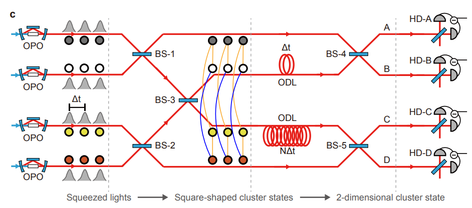
图中的三个分束器都是 \(1:1\) 分束， 同一时刻四路压缩光经过三个分束器之后在空间上形成纠缠， 然后第二路经过第一个延时线做一个周期的延时， 第三路第二个延时线圈做 \(N\) 个周期的延时( 这里\(N=5\))，最后输出的四路量子态在时间和空间上形成纠缠。 具体来说

\[ x_k^A + x_k^B - \frac{1}{\sqrt{2}}(-x^A_{k+1} + x^B_{k+1} + x^C_{k+N} + x^D_{k+N}) = 0 \]

\(k\) 对应的是时间指标。

随时间的纠缠过程如下图所示，

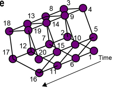
从上面的等式的前四项可以看出 \(k\) 时刻和 \(k+1\) 时刻是纠缠在一起的，这里就形成一维的纠缠链， 同时后两项增加了 \(k+N\) 时刻的纠缠， 这里就形成了二维的纠缠，具体细节可以参考[2]。

代码演示

r = 8
nmode = 4
cir = dq.QumodeCircuitTDM(nmode=nmode, init_state='vac', cutoff=3)
cir.s(0, r=r)
cir.s(1, r=r)
cir.s(2, r=r)
cir.s(3, r=r)
cir.r(0, np.pi / 2)
cir.r(2, np.pi / 2)
cir.bs([0, 1], [np.pi / 4, 0])
cir.bs([2, 3], [np.pi / 4, 0])
cir.bs([1, 2], [np.pi / 4, 0])
cir.delay(1, ntau=1, inputs=[np.pi / 2, np.pi])
cir.delay(2, ntau=5, inputs=[np.pi / 2, np.pi])
cir.bs([0, 1], [np.pi / 4, 0])
cir.bs([2, 3], [np.pi / 4, 0])
cir.homodyne_x(0, eps=1e-6)
cir.homodyne_x(1, eps=1e-6)
cir.homodyne_x(2, eps=1e-6)
cir.homodyne_x(3, eps=1e-6)
cir.to(torch.double)
cir()
cir.draw()

cir(nstep=100)

查看等效的展开后的线路

cir.draw(unroll=True)

现在运行线路100次，对采样结果做统计分析来验证

\[ x_k^A + x_k^B - \frac{1}{\sqrt{2}}(-x^A_{k+1} + x^B_{k+1} + x^C_{k+N} + x^D_{k+N}) = 0 \]

cir(nstep=100)
samples = cir.samples
samples = samples.mT
err = []
for i in range(90):
    temp = samples[i][:2].sum() - 1 / np.sqrt(2) * (-samples[i + 1][0] + samples[i + 1][1] + samples[i + 5][2:].sum())
    err.append(temp)
err = torch.tensor(err)
print('variance:', err.std() ** 2)
print('mean:', err.mean())

variance: tensor(5.4542e-07, dtype=torch.float64)
mean: tensor(-3.7434e-05, dtype=torch.float64)

附录

[1] Yokoyama S, Ukai R, Armstrong S C, et al. Ultra-large-scale continuous-variable cluster states multiplexed in the time domain[J]. Nature Photonics, 2013, 7(12): 982-986.

[2] Asavanant W. Time-Domain Multiplexed 2-Dimensional Cluster State: Universal Quantum Computing Platform[J]. arxiv. org, Cornell University Library, 201.