玻色采样(Boson Sampling)#

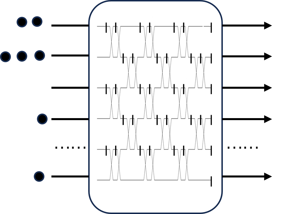
玻色采样由Aaronson和Arkhipov引入[1]，它描述了这样一个物理过程：多个全同的单光子通过线性光学器件组成的多模光量子线路相互干涉后，通过多次采样可以得到输出端口对应的概率分布，如下图所示。

同时玻色采样的概率分布可以由理论计算得到，数学上对应着积和式（permanent）的计算。

一个 \(n \times n\) 矩阵 \(A\) 的积和式的定义如下，

\[ \mathrm{Perm}(A) = \sum_{\sigma\in S_n}\prod_{i=1}^n a_{i,\sigma_i} \]

其中 \(S_n\) 为 \(n\) 阶置换群，即包含所有 \(n\) 元排列的集合，\(n=2\) 时

\[\begin{split} A= \begin{pmatrix} a_{11}&a_{12}\\ a_{21}&a_{22} \end{pmatrix}, \ \ \ \mathrm{Perm}(A) = a_{11}a_{22}+a_{12}a_{21} \end{split}\]

对玻色采样的精确模拟需要精确地求解积和式这一 \(\#P\) 难的问题。而即便在近似条件下模拟玻色采样，Aaronson 等人同样证明了其困难性。

假设输入的量子态为 \(N\) 模的Fock态 \(|\psi\rangle\)，\(|\psi\rangle = |m_1, m_2,...,m_N\rangle\), \(U\) 表示光量子线路对应的酉矩阵, 对应的生成算符变换如下:

\[(\hat{a}^+_{out})_k = \sum_{i=0}^NU_{kj}(\hat{a}^+_{in})_j\]

探测到特定的量子态组合 \(|n_1,n_2,...,n_N\rangle\) 的概率为

\[ |\langle n_1,n_2,...,n_N|W|\psi \rangle|^2 \]

这里 \(W\) 表示 \(U\) 对量子态的作用，因为在光量子线路中的酉矩阵 \(U\) 直接作用对象是生成算符和湮灭算符，所以需要 \(W\) 表示对量子态的作用，具体的，输出的振幅可以表示成

\[ \langle n_1,n_2,...,n_N|W|\psi\rangle = \frac{\mathrm{Perm}(U_{st})}{\sqrt{m_1!...m_N!n_1...n_N!}} \]

输出的概率可以写成

\[ |\langle n_1,n_2,...,n_N|W|\psi\rangle|^2 = \frac{|\mathrm{Perm}(U_{st})|^2}{m_1!...m_N!n_1...n_N!} \]

这里的 \(U_{st}\) 是通过对 \(U\) 取行取列组合来得到，具体来说，根据输入 \(|\psi\rangle = |m_1, m_2,...,m_N\rangle\) 取对应的第 \(i\) 行并且重复\(m_i\) 次，如果 \(m_i=0\) 则不取，根据输出 \(|n_1,n_2,...,n_N\rangle\) 取对应的第 \(j\) 列并且重复 \(m_j\) 次，如果 \(m_j=0\) 则不取。

比如下面的2光子玻色采样例子[2]

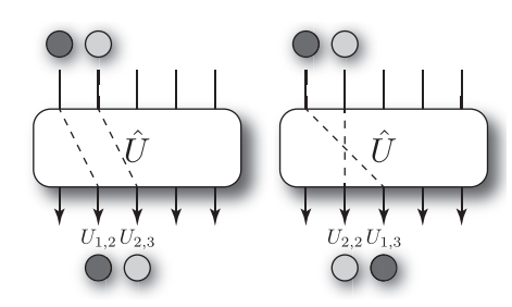
假设两个光子从1、2端口输入，那么从2、3端口输出的的概率 \(P_{2,3}\) 如下，

\[\begin{split} P_{2,3} = U_{1,2}U_{2,3} + U_{1,3}U_{2,2} =\mathrm{Perm}(U_{sub}) = \mathrm{Perm}\begin{pmatrix}U_{1,2} & U_{2,2}\\ U_{1,3} & U_{2,3}\end{pmatrix} \end{split}\]

\(U_{sub}\) 是对应的酉矩阵 \(U\) 取第1、2行和第2、3列构成的子矩阵的转置。

在量子模拟中，玻色采样可以用来模拟多体量子系统的动力学行为，玻色采样被用作证明量子计算机超越经典计算机能力的一种方式，即所谓的量子优越性。

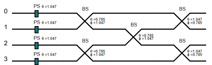
我们以下面的4模线路为例来演示玻色采样

代码示例#

## 构建一个由ps门和bs门组成的4模线路，设置初态为[1,1,0,0]
import deepquantum as dq
import numpy as np

init_state = [1, 1, 0, 0]
cir = dq.QumodeCircuit(nmode=4, init_state=init_state, backend='fock')
for k in range(4):
    cir.ps(wires=[k], inputs=np.pi / 3)
cir.bs(wires=[0, 1], inputs=[np.pi / 4, np.pi / 3])
cir.bs(wires=[2, 3], inputs=[np.pi / 4, np.pi / 3])
cir.bs(wires=[1, 2], inputs=[np.pi / 4, np.pi / 3])
cir.bs(wires=[0, 1], inputs=[np.pi / 3, np.pi / 4])
cir.bs(wires=[2, 3], inputs=[np.pi / 3, np.pi / 4])
# 线路可视化
cir.draw()

../../../_images/9047fa7728dafe101c9db49c4594d5233b27e06ecd62fdfba0c2146cf76bcfef.svg

# 线路进行演化
state = cir()
# 对演化之后的结果采样
sample = cir.measure(shots=1024)
print('final state', state)
print('sample results', sample)

final state {|1100>: tensor([0.2652-0.5714j]), |0200>: tensor([0.3709-0.2652j]), |1001>: tensor([0.1875+0.3248j]), |0002>: tensor([0.2296+0.1326j]), |0011>: tensor([0.2091-0.0560j]), |1010>: tensor([0.2091+0.0560j]), |0101>: tensor([0.0560-0.2091j]), |2000>: tensor([-0.0884+0.1121j]), |0110>: tensor([-0.0625-0.1083j]), |0020>: tensor([0.0442-0.0765j])}
sample results {|1100>: 404, |0110>: 15, |2000>: 17, |1001>: 150, |0200>: 218, |1010>: 58, |0002>: 67, |0011>: 49, |0101>: 40, |0020>: 6}

根据前面的讨论可以知道输出的概率是可以理论计算的，下面我们将分步计算输出的概率并验证

计算光量子线路对应的酉矩阵

## 计算光量子线路的酉矩阵
u_ps = np.diag([np.exp(1j * np.pi / 3), np.exp(1j * np.pi / 3), np.exp(1j * np.pi / 3), np.exp(1j * np.pi / 3)])

u_bs1 = np.array(
    [
        [np.cos(np.pi / 4), -np.exp(-1j * np.pi / 3) * np.sin(np.pi / 4)],
        [np.exp(1j * np.pi / 3) * np.sin(np.pi / 4), np.cos(np.pi / 4)],
    ]
)
u_bs1 = np.block([[u_bs1, np.zeros([2, 2])], [np.zeros([2, 2]), np.eye(2)]])

u_bs2 = np.array(
    [
        [np.cos(np.pi / 4), -np.exp(-1j * np.pi / 3) * np.sin(np.pi / 4)],
        [np.exp(1j * np.pi / 3) * np.sin(np.pi / 4), np.cos(np.pi / 4)],
    ]
)
u_bs2 = np.block([[np.eye(2), np.zeros([2, 2])], [np.zeros([2, 2]), u_bs2]])

u_bs3 = np.array(
    [
        [np.cos(np.pi / 4), -np.exp(-1j * np.pi / 3) * np.sin(np.pi / 4)],
        [np.exp(1j * np.pi / 3) * np.sin(np.pi / 4), np.cos(np.pi / 4)],
    ]
)
u_bs3 = np.block([[1, np.zeros(2), 0], [np.zeros([2, 1]), u_bs3, np.zeros([2, 1])], [0, np.zeros(2), 1]])

u_bs4 = np.array(
    [
        [np.cos(np.pi / 3), -np.exp(-1j * np.pi / 4) * np.sin(np.pi / 3)],
        [np.exp(1j * np.pi / 4) * np.sin(np.pi / 3), np.cos(np.pi / 3)],
    ]
)
u_bs4 = np.block([[u_bs4, np.zeros([2, 2])], [np.zeros([2, 2]), np.eye(2)]])

u_bs5 = np.array(
    [
        [np.cos(np.pi / 3), -np.exp(-1j * np.pi / 4) * np.sin(np.pi / 3)],
        [np.exp(1j * np.pi / 4) * np.sin(np.pi / 3), np.cos(np.pi / 3)],
    ]
)
u_bs5 = np.block([[np.eye(2), np.zeros([2, 2])], [np.zeros([2, 2]), u_bs5]])

u_total = u_bs5 @ u_bs4 @ u_bs3 @ u_bs2 @ u_bs1 @ u_ps

计算输出结果及对应的子矩阵

out_state = [1, 1, 0, 0]
u_sub = u_total[:2][:, :2]
print(u_sub)

[[ 0.06470476-0.11207193j -0.77181154-0.11207193j]
 [-0.28349365+0.8080127j  -0.3080127 -0.21650635j]]

计算子矩阵对应的permanent可以得到对应概率

per = u_sub[0, 0] * u_sub[1, 1] + u_sub[0, 1] * u_sub[1, 0]
amp = per
prob = abs(per) ** 2
print(amp, state[dq.FockState(out_state)])

(0.2651650429449553-0.5713512607928528j) tensor([0.2652-0.5714j])

附录#

[1] Scott Aaronson and Alex Arkhipov. The computational complexity of linear optics. Theory of Computing, 9(1):143–252, 2013. doi:10.4086/toc.2013.v009a004.

[2] Gard, B. T., Motes, K. R., Olson, J. P., Rohde, P. P., & Dowling, J. P. (2015). An introduction to boson-sampling. In From atomic to mesoscale: The role of quantum coherence in systems of various complexities (pp. 167-192).

玻色采样(Boson Sampling)

Contents

玻色采样(Boson Sampling)#

代码示例#

附录#