混合量子经典循环神经网络

搭建量子RNN网络

本节内容将详细介绍混合量子经典循环神经网络（Quantum Recurrent Neural Network，简称 QRNN）的构建过程，并展示其在量子模拟器上的模型架构与实验效果[1] [2]。混合量子经典循环神经网络是传统循环神经网络（Recurrent Neural Network，简称 RNN）的量子化版本，其主要特点在于将 RNN 单元中的全连接层替换为变分量子线路（Variational Quantum Circuit，简称 VQC），同时保留了单元中原有的计算逻辑。通过本节的学习，您将深入理解混合量子经典循环神经网络的基础理论、实现方法，以及在解决实际问题时的应用案例。在探究量子RNN模型的搭建之前，首先需了解其核心组成部分——变分量子线路（Variational Quantum Circuit, VQC）。变分量子线路（VQC），也被称为参数化量子线路（Parameterized Quantum Circuit, PQC），通常包含三个关键部分：状态制备、变分量子线路和测量。下图中 \(U(x)\) 表示状态制备线路，它的作用是将经典数据 \(x\) 编码为量子态。 \(V(\theta)\) 表示具有可调节参数 \(\theta\) 的变分线路，可以通过梯度下降的方法进行优化。最后通过测量量子态，得到经典的输出值[1] [2]。

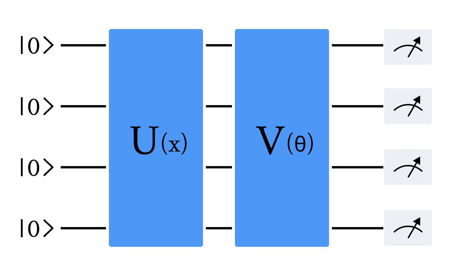
图 1 变分量子线路（VQC）的通用架构。U(x) 是将经典输入数据 x 编码为量子态的量子线路，V(θ) 是具有可调节或可学习参数 θ 的变分线路。线路最后是对部分或全部量子比特的测量

在这里，我们通过 DeepQuantum 去实现一个用于 QRNN 的 VQC 模块（图1），包括以下三个部分： 编码线路、变分线路和量子测量。

1.编码线路

编码线路将经典数据值映射为量子振幅。量子线路先进行基态初始化，然后利用 Hadamard 门来制备无偏初始态。我们使用双角编码（two-angle encoding），用两个角度编码一个值，将每个数据值分别用两个量子门（ Ry 和 Rz ）进行编码。两个量子门的旋转角度分别为：\( f(x _i) = \arctan(x _i) \) 和 \( g(x _i) = \arctan(x _i^2) \) ，其中 \( x _i \) 是数据向量 \( x \) 的一个分量。编码数据的量子态为[1]：

\[ |x\rangle=\bigotimes^N_{i=1}\cos(f(x_i)+\pi/4)|0\rangle+\exp(ig(x_i))\sin(f(x_i)+\pi/4)|1\rangle \]

其中 N 是向量 \( x \) 的维数，\(\pi /4\) 的角偏移是因为初始的 Hadamard 门旋转。

2.变分线路

变分量子线路由几个 CNOT 门和单量子比特旋转门组成。CNOT门以循环的方式作用于每一对位置距离1和2的量子比特，用于产生纠缠量子比特。可学习参数 \(\alpha\) ， \(\beta\) 和 \(\gamma\) 控制单量子比特旋转门，它们可以基于梯度下降算法进行迭代优化更新。该变分量子线路模块可以重复多次，以增加变分参数的数量。

3.量子测量

VQC块的末端是一个量子测量层，我们通过测量来计算每个量子态的期望值。在量子模拟软件中，我们可以在经典计算机上进行数值计算，而在真实的量子计算机中，这些数值是通过重复测量进行统计估计得到的。

# 首先我们导入所有需要的包：
import torch
import torch.nn as nn
import deepquantum as dq
import matplotlib.pyplot as plt
import numpy as np
from torch.utils.data import Dataset
from torch.utils.data import DataLoader
import pandas as pd

# 我们设计的VQC线路如下 这里我们以4个bit作为例子
cir = dq.QubitCircuit(4)
cir.hlayer()
cir.rylayer(encode=True)
cir.rzlayer(encode=True)
cir.barrier()
cir.cnot_ring()
cir.barrier()
cir.cnot_ring(step=2)
cir.barrier()
cir.u3layer()
cir.barrier()
cir.measure()
cir.draw() # 画出量子线路图

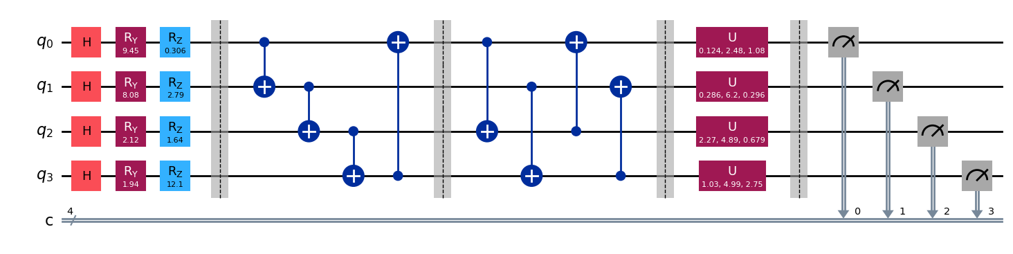
VQC 模块由三个主要部分构成：编码线路、变分线路以及量子测量。编码线路包含 H 门、Ry 门和 Rz 门，负责将信息编码至量子态。变分线路位于第1条和第4条虚线之间，其结构可以根据需要调整。量子比特的数量和量子测量的次数均可按实验需求进行灵活配置。此外，变分线路的层数和参数数量可以增加，以扩展模型规模，这主要取决于所使用的量子计算机或量子模拟软件的处理能力。在本节的示例中，所用的量子比特数量为4个。

量子RNN模型

在讲解量子 RNN 模型前，我们先简单回顾一下经典 RNN 模型的原理和结构（图2）。我们使用数学公式描述经典 RNN 模型的计算单元：

\[ h_t = \tanh(x_t W_{ih}^T + b_{ih} + h_{t-1}W_{hh}^T + b_{hh}) \]

其中 \( W_{ih} \) 是作用在 \( x_t \) 上的隐藏层权重参数， \( b_{ih} \) 是对应的隐藏层偏差参数， \( W_{hh} \) 是作用在 \( h_{t-1} \) 上的隐藏层权重参数， \( b_{hh} \) 是对应的隐藏层偏差参数，这里使用 tanh 函数作为激活函数。

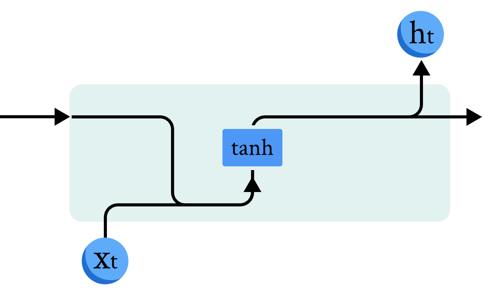
图 2 经典RNN模型示意图

量子 RNN 模型是经典 RNN 模型的量子版本。主要区别在于经典神经网络被 VQC 取代，我们使用数学公式描述 QRNN 模型的计算单元 [1]：

\[ h_t = \tanh(VQC(v_t)) \]

\[ y_t = NN(h_t) \]

其中输入 \( v_t \) 是前一个时间步长的隐藏状态 \( h_{t−1} \) 与当前输入向量 \( x_t \) 的级联， \( NN \) 是经典神经网络层。

首先我们先用DeepQuantum实现一个VQC模块：

## 定义VQC模块
class QuLinear(nn.Module):
    def __init__(self, input_size, hidden_size):
        super(QuLinear, self).__init__()
        n_qubits = input_size  #定义比特个数
        self.cir = dq.QubitCircuit(n_qubits, reupload=True)
        self.cir.hlayer()
        self.cir.rylayer(encode=True)
        self.cir.rzlayer(encode=True)
        self.cir.barrier()
        self.cir.cnot_ring()
        self.cir.barrier()
        self.cir.cnot_ring(step=2)
        self.cir.barrier()
        self.cir.u3layer()

        self.cir.barrier()     #两层变分线路模块[1]
        self.cir.cnot_ring()
        self.cir.barrier()
        self.cir.cnot_ring(step=2)
        self.cir.barrier()
        self.cir.u3layer()


        for i in range(hidden_size): # 以for循环
            self.cir.observable(wires=i, basis='z')

    def forward(self, x):
        ry_parameter = torch.arctan(x)   #将经典数据转化为对应ry的角度
        rz_parameter = torch.arctan(x*x) #将经典数据转化为对应rz的角度
        r_parameter=torch.cat([ry_parameter,rz_parameter],dim=1)
        self.cir(r_parameter)
        return self.cir.expectation()

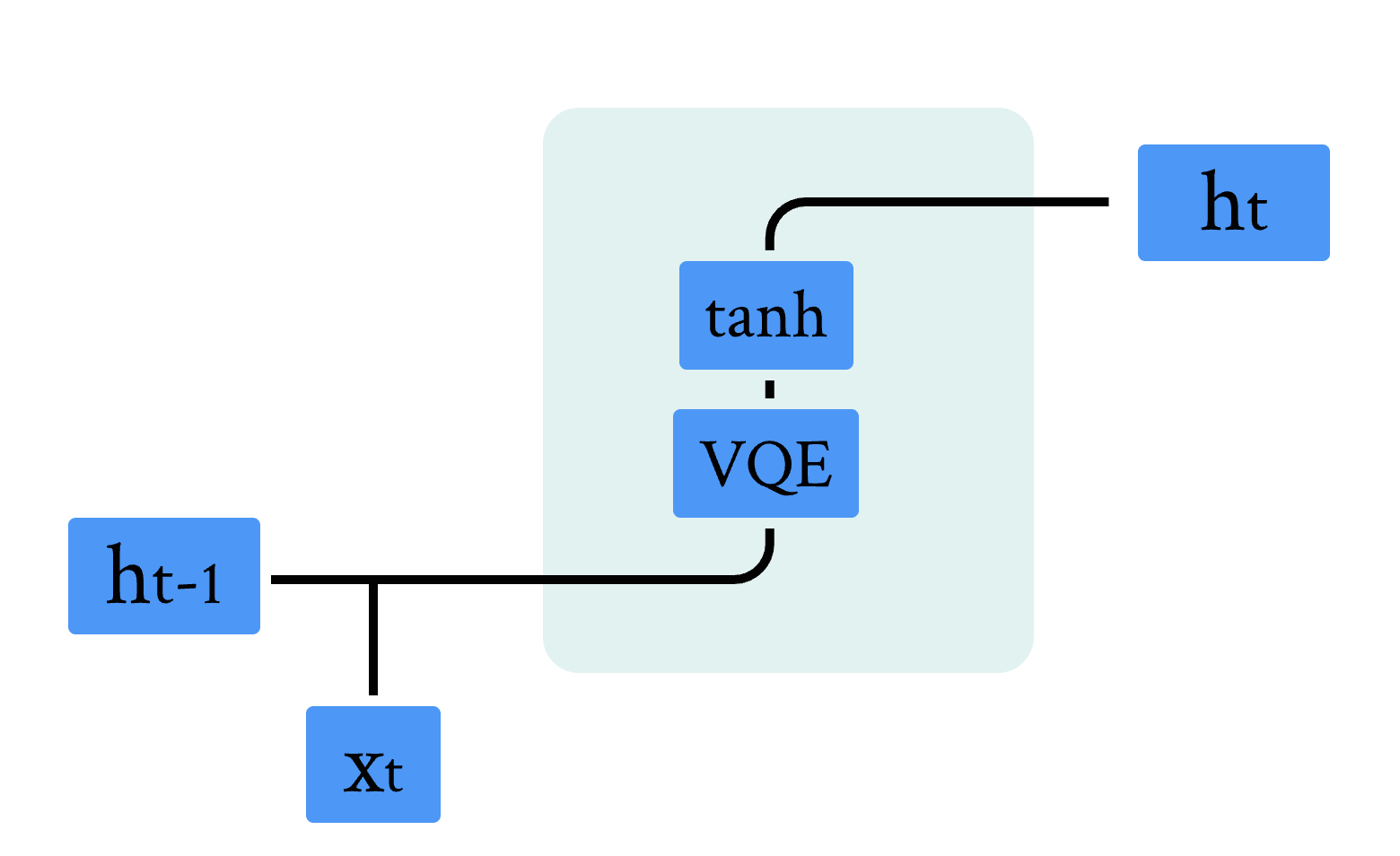
图 3 量子RNN模型示意图

图 3 展示了混合量子经典 RNN 的单元结构，结合前面章节的内容，不难发现，相比于经典结构，其中的线性全连接层被 VQC 线路替换，我们可以利用上面我们实现的 QuLinear，结合经典 RNN 的计算逻辑，实现量子混合经典循环神经网络。代码如下：

class QRNNCell(nn.Module):
    def __init__(self, input_size, hidden_size):
        super(QRNNCell, self).__init__()

        self.input_size = input_size
        self.hidden_size = hidden_size
        self.linear = QuLinear(input_size+hidden_size, hidden_size)
        self.tanh = nn.Tanh()
    def forward(self, x, h):
        v = torch.cat((x, h), dim=-1)
        h = self.tanh(self.linear(v))
        return h


class QRNN_hybrid(nn.Module):
    def __init__(self, input_size, hidden_size, target_size, device):
        super(QRNN_hybrid, self).__init__()
        self.input_size = input_size
        self.hidden_size = hidden_size
        self.h0_linear = nn.Linear(hidden_size, hidden_size)
        self.gru = QRNNCell(input_size, hidden_size)
        self.tanh = nn.Tanh()
        self.device = device
        self.predictor = nn.Linear(hidden_size, target_size)

    def forward(self, x, hidden_state=None):
        # 初始化隐藏状态
        if hidden_state is None:
            batch_size, sequence_length, _ = x.size()
            h0 = self.tanh(self.h0_linear(torch.zeros(batch_size, self.hidden_size).to(self.device))).to(self.device)
            # 存储所有时间步的隐藏状态
            hidden_states = []
            # 遍历所有时间步
            for t in range(sequence_length):
                xt = x[:, t, :]
                ht = self.gru(xt, h0)
                hidden_states.append(ht.unsqueeze(1))
                h0 = ht
            output = self.predictor(torch.cat(hidden_states, dim=1))
            return output, hidden_states[-1]
        else:
            ht = self.gru(x[:, -1].unsqueeze(1), hidden_state)
            output = self.predictor(ht)
            return output, ht

# 测试模型代码能否成功运行
# 定义输入、隐藏状态和输出的维度
input_size = 2   #输入
hidden_size = 3
output_size = 1  #输出一个数值
# 创建模型实例
device = torch.device("cpu")
model = QRNN_hybrid(input_size, hidden_size, output_size, device)
# 随机生成输入数据
batch_size = 3
sequence_length = 4
input_data = torch.randn(batch_size, sequence_length, input_size)
# 前向传播
output, _ = model(input_data)
# 输出结果
print("输出的形状:", output.shape)

输出的形状: torch.Size([3, 4, 1])

量子RNN模型训练

本节将介绍量子 RNN 模型训练过程，包括训练的数据介绍，训练过程的代码实现。

数据任务

在这里，我们使用余弦函数作为模型训练的数据集，首先定义数据集构建函数，代码如下：

#构建时间序列数据集
class TimeSeriesDataset(Dataset):
    def __init__(self, data, sequence_length):
        self.data = data
        self.sequence_length = sequence_length   #定义数据长度
        self.xdata = []
        self.ydata = []
        for i in range(len(data)):
            if i + self.sequence_length + 1 > len(data):
                break
            self.xdata.append(self.data[i:i+self.sequence_length])      #xdata为输入数据
            self.ydata.append(self.data[i+1:i+self.sequence_length+1])  #ydata为需要预测的后一位输出数据

    def __len__(self):
        return len(self.xdata)

    def __getitem__(self, index):
        x = self.xdata[index]
        y = self.ydata[index]  # 目标序列错开一位
        return x, y

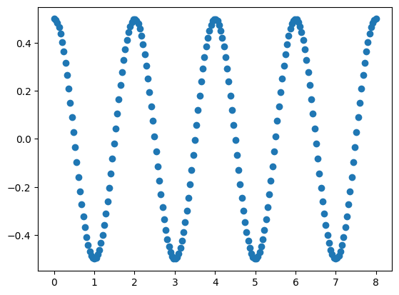
我们给出范围在 \([0, 8\pi]\) 的余弦函数，振幅为0.5，将其分为200个数据点，取前100个数据点作为模型的训练数据，代码如下：

start = 0
end = 8
data_points = 200
amplitude = 0.5
num_train_points = 100

time_steps = np.linspace(start, end, data_points) # 在区间[0, 8*pi]之间线性均匀的选择200个数据点
data = np.cos(np.pi*time_steps)*amplitude # 生成区间[0, 8*pi]上的余弦信号时间序列数据
train_data = data[:num_train_points] # 选择前100个数据点作为训练集
test_data = data[num_train_points:]
# 创建数据集对象
# 由于第一个数据点不需要预测 而序列的最后一个数据点不能出现在训练的输入特征中 这里特征序列和标签序列的长度都需要设为总长度-1
sequence_length = num_train_points - 1
dataset = TimeSeriesDataset(torch.tensor(train_data), sequence_length)
# 创建数据加载器
# 这里我们不做数据的窗口切分，因此每个batch中只有一条完整数据，并且只有一个batch
batch_size = 1
dataloader = DataLoader(dataset, batch_size=batch_size)

#画出我们的数据集
plt.plot(time_steps, data,'o')
plt.show()

全参数训练

在接下来的实验中，我们将利用上一小节中准备的数据集，以及基于上一节构建的 QRNN 模型来进行模型训练。实验中采用均方差损失函数（Mean Squared Error Loss，简称 MSELoss）作为训练过程中的损失函数。选用的优化器为 RMSprop[1]，这是一种基于梯度下降法的变体，它具备自适应学习率调整的特性。优化器的超参数配置如下：平滑常数alpha设为0.99，eps设为1e−8，动量（momentum）设为0.5。下面是定义模型训练函数的代码：

def trainer(model, epoch, learning_rate, device):
    criterion = nn.MSELoss()
    optimizer = torch.optim.RMSprop(model.parameters(),learning_rate,alpha=0.99,eps=1e-08,weight_decay=0,momentum=0.5,centered=False)

    model = model.to(device)
    flag = False
    train_loss_list=[]

    for e in range(epoch):
        if flag:
            break
        for x, y in dataloader:
            x = x.unsqueeze(-1).float()
            y = y.unsqueeze(-1).float()
            x = x.to(device)
            y = y.to(device)
            y_pred, _ = model(x)
            loss = criterion(y_pred, y)
            optimizer.zero_grad()
            loss.backward()
            optimizer.step()
        train_loss_list.append(loss.detach().numpy())
        print("Iteration: {} loss {}".format(e, loss.item()))

    metrics = {'epoch': list(range(1, len(train_loss_list)+1)),
                'train_loss': train_loss_list}
    return model, metrics

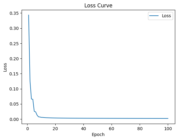
我们设置优化器的学习率 lr 为0.01，迭代次数为100次，模型中 VQC 的输入量子比特个数为1，隐藏层量子比特个数为3，输出量子比特个数为1。分别训练 QRNN，QLSTM 和 QGRU 模型，代码如下：

# 训练混合量子经典RNN
lr = 0.01   #定义学习率为0.01
epoch = 100 #定义迭代次数为100次
device = torch.device("cpu")
model_QRNN = QRNN_hybrid(1, 3, 1, device)

optim_model, metrics=trainer(model_QRNN, epoch, lr, device)

Iteration: 0 loss 0.34345731139183044
Iteration: 1 loss 0.12530270218849182
Iteration: 2 loss 0.06626231968402863
Iteration: 3 loss 0.0652255117893219
Iteration: 4 loss 0.025696925818920135
Iteration: 5 loss 0.023623822256922722
Iteration: 6 loss 0.013093587942421436
Iteration: 7 loss 0.007445588242262602
Iteration: 8 loss 0.006811297498643398
Iteration: 9 loss 0.005624251440167427
Iteration: 10 loss 0.005475181620568037
Iteration: 11 loss 0.004980004858225584
Iteration: 12 loss 0.004626949783414602
Iteration: 13 loss 0.0043708560988307
Iteration: 14 loss 0.004152844659984112
Iteration: 15 loss 0.003995758481323719
Iteration: 16 loss 0.0038470348808914423
Iteration: 17 loss 0.003717939369380474
Iteration: 18 loss 0.0036027433816343546
Iteration: 19 loss 0.0035006145481020212
Iteration: 20 loss 0.003411721671000123
Iteration: 21 loss 0.00333323422819376
Iteration: 22 loss 0.003263943362981081
Iteration: 23 loss 0.0032021738588809967
Iteration: 24 loss 0.003146733855828643
Iteration: 25 loss 0.0030966445337980986
Iteration: 26 loss 0.0030510765500366688
Iteration: 27 loss 0.0030094003304839134
Iteration: 28 loss 0.0029710703529417515
Iteration: 29 loss 0.002935644704848528
Iteration: 30 loss 0.0029027434065937996
Iteration: 31 loss 0.002872057957574725
Iteration: 32 loss 0.002843312919139862
Iteration: 33 loss 0.002816280350089073
Iteration: 34 loss 0.002790765604004264
Iteration: 35 loss 0.0027666029054671526
Iteration: 36 loss 0.0027436381205916405
Iteration: 37 loss 0.002721746452152729
Iteration: 38 loss 0.0027008187025785446
Iteration: 39 loss 0.0026807545218616724
Iteration: 40 loss 0.0026614745147526264
Iteration: 41 loss 0.002642899751663208
Iteration: 42 loss 0.0026249708607792854
Iteration: 43 loss 0.002607630332931876
Iteration: 44 loss 0.00259082717821002
Iteration: 45 loss 0.0025745187886059284
Iteration: 46 loss 0.0025586693082004786
Iteration: 47 loss 0.002543241949751973
Iteration: 48 loss 0.002528208075091243
Iteration: 49 loss 0.0025135399773716927
Iteration: 50 loss 0.0024992208927869797
Iteration: 51 loss 0.0024852235801517963
Iteration: 52 loss 0.0024715287145227194
Iteration: 53 loss 0.0024581244215369225
Iteration: 54 loss 0.002444991609081626
Iteration: 55 loss 0.002432123525068164
Iteration: 56 loss 0.002419498283416033
Iteration: 57 loss 0.0024071133229881525
Iteration: 58 loss 0.002394952578470111
Iteration: 59 loss 0.002383013954386115
Iteration: 60 loss 0.002371283248066902
Iteration: 61 loss 0.0023597567342221737
Iteration: 62 loss 0.0023484269622713327
Iteration: 63 loss 0.002337286714464426
Iteration: 64 loss 0.0023263278417289257
Iteration: 65 loss 0.0023155531380325556
Iteration: 66 loss 0.0023049493320286274
Iteration: 67 loss 0.0022945119999349117
Iteration: 68 loss 0.0022842413745820522
Iteration: 69 loss 0.0022741290740668774
Iteration: 70 loss 0.0022641755640506744
Iteration: 71 loss 0.00225437106564641
Iteration: 72 loss 0.00224471976980567
Iteration: 73 loss 0.0022352132946252823
Iteration: 74 loss 0.002225845819339156
Iteration: 75 loss 0.0022166199050843716
Iteration: 76 loss 0.0022075290326029062
Iteration: 77 loss 0.0021985704079270363
Iteration: 78 loss 0.0021897449623793364
Iteration: 79 loss 0.0021810452453792095
Iteration: 80 loss 0.002172466367483139
Iteration: 81 loss 0.0021640132181346416
Iteration: 82 loss 0.0021556788124144077
Iteration: 83 loss 0.002147459192201495
Iteration: 84 loss 0.002139358315616846
Iteration: 85 loss 0.0021313640754669905
Iteration: 86 loss 0.002123478800058365
Iteration: 87 loss 0.0021157003939151764
Iteration: 88 loss 0.0021080244332551956
Iteration: 89 loss 0.0021004509180784225
Iteration: 90 loss 0.00209297938272357
Iteration: 91 loss 0.0020856026094406843
Iteration: 92 loss 0.0020783196669071913
Iteration: 93 loss 0.0020711275283247232
Iteration: 94 loss 0.0020640259608626366
Iteration: 95 loss 0.0020570168271660805
Iteration: 96 loss 0.002050088020041585
Iteration: 97 loss 0.0020432458259165287
Iteration: 98 loss 0.002036480000242591
Iteration: 99 loss 0.002029797527939081

# 绘制QRNN模型的loss曲线
epoch = metrics['epoch']
loss = metrics['train_loss']

# 创建图和Axes对象
# 绘制训练损失曲线
plt.plot(epoch, loss, label='Loss')
plt.title('Loss Curve')
plt.xlabel('Epoch')
plt.ylabel('Loss')
plt.legend()

<matplotlib.legend.Legend at 0x20c085b33d0>

参考文献

[1] Chen, S. Y. C., Fry, D., Deshmukh, A., Rastunkov, V., & Stefanski, C. (2022). Reservoir computing via quantum recurrent neural networks. arXiv preprint arXiv:2211.02612.

[2] Chen, S. Y. C., Yoo, S., & Fang, Y. L. L. (2022, May). Quantum long short-term memory. In ICASSP 2022-2022 IEEE International Conference on Acoustics, Speech and Signal Processing (ICASSP) (pp. 8622-8626). IEEE.